Balancing distributions for observational studies

Theory

Distributional entropy balancing

Our proposal, which leads to distributional entropy balancing (hereinafter DEB), is based on extending the original idea by adding additional constraint(s) on the weights on \(\mathbf{a}_k\), as presented below.

\[ \begin{aligned} \max _{w} H(w)=- & \sum_{k \in s_0} v_{k} \log \left(v_{k} / q_{k}\right), \\ \text { s.t. } & \sum_{k \in s_0} v_{k} G_{k j}=m_{k} \text { for } j \in 1, \ldots, J_1, \\ & \sum_{k \in s_0} v_{k} a_{k j}=\frac{\alpha_{j}}{n_1} \text { for } j \in 1, \ldots, J_2, \\ & \sum_{k \in s_0} v_{k}=1 \text { and } v \geq 0 \text { for all } k \in s_0. \end{aligned} \]

Distributional propensity score method

(imai2014covariate?) proposed covariate balancing propensity score (CBPS) to estimate the (eqref?){eq-ate}, where unknown parameters of the propensity score model \(\mathbf{\gamma}\) are estimated using the generalized method of moments as

\[ \mathbb{E}\left[\left(\frac{\mathcal{D}}{p\left(\mathbf{X}; \mathbf{\gamma}\right)}-\frac{1-\mathcal{D}}{1-p\left(\mathbf{X}; \mathbf{\gamma}\right)}\right) f(\mathbf{X})\right]=\mathbf{0}, \label{eq-cbps} \]

where \(p()\) is the propensity score. This balances means of the the \(\mathbf{X}\) variables, which may not be sufficient if the variables are highly skewed or we are interested in estimating DTE or QTE.

We propose a simple approach based on the specification of moments and \(\alpha\)-quantiles to be balanced. Instead of using the matrix \(\mathbf{X}\), we propose to use the matrix \(\mathcal{X}\), which is constructed as follows

\[ \mathcal{X} = \begin{bmatrix} \mathbf{1}^1 & \mathbf{X}^1 & \mathbf{A}^1\\ \mathbf{1}^0 & \mathbf{X}^0 & \mathbf{A}^0\\ \end{bmatrix}, \]

where \(\mathbf{X}^0, \mathbf{X}^1\) are matrices of size \(n_0 \times J_1\) and \(n_1 \times J_1\) with \(J_1\) covariates to be balanced at the means, and \(\mathbf{A}^1, \mathbf{A}^0\) are matrices with are based on \(J_2\) covariates with elements defined as follows

\[ a^1_{kj}=\left\{\begin{array}{lll} n_1^{-1},& \quad x_{kj}^1\leq L_{x_{j},1}\left(q^1_{x_{j},\alpha}\right),\\ n_1^{-1}\beta_{x_{j},1}\left(q^1_{x_{j},\alpha}\right), & \quad x_{kj}^1=U_{x_{j},1}\left(q^1_{x_{j},\alpha}\right),\\ 0,& \quad x^1_{kj}> U_{x_{j},1}\left(q^1_{x_{j},\alpha}\right),\\ \end{array} \right. \]

and

\[ a^0_{kj}=\left\{\begin{array}{lll} n_1^{-1},& \quad x_{kj}^0\leq L_{x_{j},0}\left(q^1_{x_{j},\alpha}\right),\\ n_1^{-1}\beta_{x_{j},0}\left(q^1_{x_{j},\alpha}\right), & \quad x_{kj}^0=U_{x_{j},0}\left(q^1_{x_{j},\alpha}\right),\\ 0,& \quad x^0_{kj}> U_{x_{j},0}\left(q^1_{x_{j},\alpha}\right),\\ \end{array} \right. \]

where \(n_1\) is the size of the treatment group, or alternatively the logistic function \(\eqref{eq-logistic-a}\) can be used.

Packages

Load packages for the example

library(jointCalib)
library(CBPS)
#> Loading required package: MASS
#> Loading required package: MatchIt
#> Loading required package: nnet
#> Loading required package: numDeriv
#> Loading required package: glmnet
#> Loading required package: Matrix
#> Loaded glmnet 4.1-8
#> CBPS: Covariate Balancing Propensity Score
#> Version: 0.23
#> Authors: Christian Fong [aut, cre],
#>   Marc Ratkovic [aut],
#>   Kosuke Imai [aut],
#>   Chad Hazlett [ctb],
#>   Xiaolin Yang [ctb],
#>   Sida Peng [ctb],
#>   Inbeom Lee [ctb]
library(ebal)
#> ##
#> ## ebal Package: Implements Entropy Balancing.
#> ## See http://www.stanford.edu/~jhain/ for additional information.
library(laeken)

Read the the LaLonde data from the CBPS package.

data("LaLonde", package = "CBPS")
head(LaLonde)
#>     exper treat age educ black hisp married nodegr re74 re75 re78 re74.miss
#> 298     0     0  47   12     0    0       0      0    0    0    0         0
#> 299     0     0  50   12     1    0       1      0    0    0    0         1
#> 300     0     0  44   12     0    0       0      0    0    0    0         0
#> 301     0     0  28   12     1    0       1      0    0    0    0         1
#> 302     0     0  54   12     0    0       1      0    0    0    0         1
#> 303     0     0  55   12     0    1       1      0    0    0    0         1

ATT with entropy balancing and other methods

Single variable: `age`

First, we start with the age variable. Below we can find the distribution of age in the control and treatment group.

dens0 <- density(LaLonde$age[LaLonde$treat == 0])
dens1 <- density(LaLonde$age[LaLonde$treat == 1])
plot(dens0, main="Distribution of age", xlab="Age", ylim=c(0, max(dens0$y, dens1$y)), col = "blue")
lines(dens1, lty=2, col="red")
legend("topright", legend=c("Control", "Treatment"), lty=c(1,2), col=c("blue", "red"))

Basic descriptive statistics are given below.

aggregate(age ~ treat, data = LaLonde, FUN = quantile)
#>   treat age.0% age.25% age.50% age.75% age.100%
#> 1     0   17.0    25.0    31.0    42.5     55.0
#> 2     1   17.0    20.0    23.0    27.0     49.0

Nowe, let’s use ebal::ebalance and jointCalib::joint_calib_att with method eb (it uses uses ebal package as backend). For DEB we use deciles probs = seq(0.1, 0.9, 0.1) and balance mean as well (formula_means = ~ age). The output informs that about the target (totals) quantiles and difference between balanced and the target quantities (column precision).

bal_standard <- ebalance(LaLonde$treat, X = LaLonde[, "age"])
#> Converged within tolerance
bal_quant <- joint_calib_att(formula_means = ~ age, 
                             formula_quantiles = ~ age, 
                             treatment =  ~ treat, 
                             data = LaLonde, 
                             probs = seq(0.1, 0.9, 0.1),
                             method = "eb")
bal_quant
#> Weights calibrated using: eb with ebal backend.
#> Summary statistics for g-weights:
#>     Min.  1st Qu.   Median     Mean  3rd Qu.     Max. 
#> 0.007665 0.022555 0.046914 0.101888 0.194177 0.605874 
#> Totals and precision (abs diff: 0.1299956)
#>          totals    precision
#> N         297.0 2.632778e-03
#> age 0.10    0.1 1.688971e-10
#> age 0.20    0.2 3.377950e-10
#> age 0.30    0.3 5.067252e-10
#> age 0.40    0.4 3.901260e-09
#> age 0.50    0.5 6.496023e-09
#> age 0.60    0.6 1.144491e-08
#> age 0.70    0.7 3.277056e-08
#> age 0.80    0.8 5.172449e-08
#> age 0.90    0.9 1.811425e-07
#> age      7314.0 1.273625e-01

Compare weighted distributions with treatment group distribution.

dens0 <- density(LaLonde$age[LaLonde$treat == 0], weights = bal_standard$w/sum(bal_standard$w))
#> Warning in density.default(LaLonde$age[LaLonde$treat == 0], weights =
#> bal_standard$w/sum(bal_standard$w)): Selecting bandwidth *not* using 'weights'
dens1 <- density(LaLonde$age[LaLonde$treat == 0], weights = bal_quant$g/sum(bal_quant$g))
#> Warning in density.default(LaLonde$age[LaLonde$treat == 0], weights =
#> bal_quant$g/sum(bal_quant$g)): Selecting bandwidth *not* using 'weights'
dens2 <- density(LaLonde$age[LaLonde$treat == 1])
plot(dens0, main="Distribution of age", xlab="Age", ylim=c(0, max(dens0$y, dens1$y)))
lines(dens1, lty=2, col="blue")
lines(dens2, lty=3, col="red")
legend("topright", 
       legend=c("EB", "DEB", "Treatment"), 
       lty=c(1,2, 3), 
       col=c("black", "blue", "red"))

Compare balancing weights.

plot(x = bal_standard$w,
     y = bal_quant$g, 
     xlab = "EB", ylab = "DEB", main = "Comparison of EB and DEB weights",
     xlim = c(0, 0.7), ylim = c(0, 0.7))

More variables

Now, consider three variables: married, age and educ.

dens0 <- density(LaLonde$educ[LaLonde$treat == 0])
dens1 <- density(LaLonde$educ[LaLonde$treat == 1])
plot(dens0, main="Distribution of education", xlab="Education", ylim=c(0, max(dens0$y, dens1$y)), col = "blue")
lines(dens1, lty=2, col="red")
legend("topleft", legend=c("Control", "Treatment"), lty=c(1,2), col=c("blue", "red"))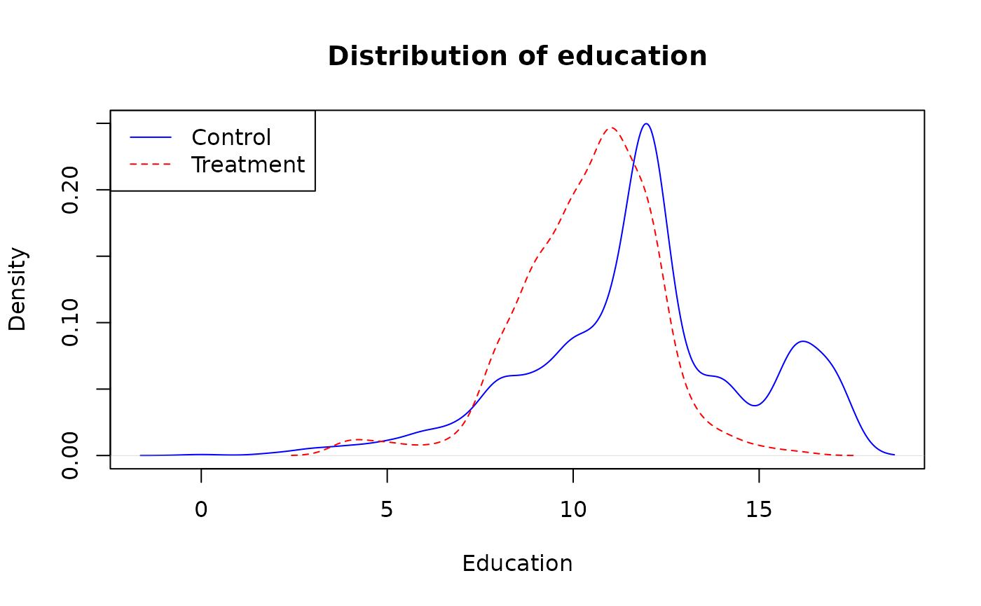

The code below balances control and treatment group on age and educ means and quantiles.

bal_standard <- ebalance(LaLonde$treat, X = LaLonde[, c("married", "age", "educ")])
#> Converged within tolerance
bal_quant <- joint_calib_att(formula_means = ~ married + age + educ, 
                             formula_quantiles = ~ age + educ, 
                             treatment =  ~ treat, 
                             data = LaLonde, 
                             method = "eb")
bal_quant
#> Weights calibrated using: eb with ebal backend.
#> Summary statistics for g-weights:
#>      Min.   1st Qu.    Median      Mean   3rd Qu.      Max. 
#> 0.0003863 0.0075341 0.0258057 0.1018874 0.0606804 2.8081281 
#> Totals and precision (abs diff: 0.08993871)
#>            totals    precision
#> N          297.00 1.646454e-03
#> age 0.25     0.25 6.697796e-08
#> age 0.50     0.50 1.541813e-07
#> age 0.75     0.75 4.802355e-07
#> educ 0.25    0.25 2.806495e-06
#> educ 0.50    0.50 3.414877e-06
#> educ 0.75    0.75 4.188730e-06
#> married     50.00 8.466613e-04
#> age       7314.00 7.261357e-02
#> educ      3083.00 1.482091e-02

Compare distribution education (educ) variable.

dens0 <- density(LaLonde$educ[LaLonde$treat == 0], weights = bal_standard$w/sum(bal_standard$w))
#> Warning in density.default(LaLonde$educ[LaLonde$treat == 0], weights =
#> bal_standard$w/sum(bal_standard$w)): Selecting bandwidth *not* using 'weights'
dens1 <- density(LaLonde$educ[LaLonde$treat == 0], weights = bal_quant$g/sum(bal_quant$g))
#> Warning in density.default(LaLonde$educ[LaLonde$treat == 0], weights =
#> bal_quant$g/sum(bal_quant$g)): Selecting bandwidth *not* using 'weights'
dens2 <- density(LaLonde$educ[LaLonde$treat == 1])
plot(dens0, main="Distribution of Education", xlab="Education", ylim=c(0, max(dens0$y, dens1$y)))
lines(dens1, lty=2, col="blue")
lines(dens2, lty=3, col="red")
legend("topleft", 
       legend=c("EB", "DEB", "Treatment"), 
       lty=c(1,2, 3), 
       col=c("black", "blue", "red"))

Compare distribution age (age) variable.

dens0 <- density(LaLonde$age[LaLonde$treat == 0], weights = bal_standard$w/sum(bal_standard$w))
#> Warning in density.default(LaLonde$age[LaLonde$treat == 0], weights =
#> bal_standard$w/sum(bal_standard$w)): Selecting bandwidth *not* using 'weights'
dens1 <- density(LaLonde$age[LaLonde$treat == 0], weights = bal_quant$g/sum(bal_quant$g))
#> Warning in density.default(LaLonde$age[LaLonde$treat == 0], weights =
#> bal_quant$g/sum(bal_quant$g)): Selecting bandwidth *not* using 'weights'
dens2 <- density(LaLonde$age[LaLonde$treat == 1])
plot(dens0, main="Distribution of age", xlab="Age", ylim=c(0, max(dens0$y, dens1$y)))
lines(dens1, lty=2, col="blue")
lines(dens2, lty=3, col="red")
legend("topright", 
       legend=c("EB", "DEB", "Treatment"), 
       lty=c(1,2, 3), 
       col=c("black", "blue", "red"))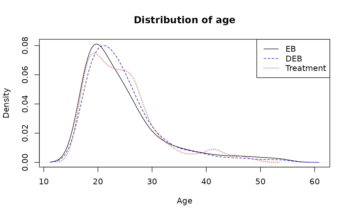

Compare balancing weights.

plot(x = bal_standard$w,
     y = bal_quant$g, 
     xlab = "EB", ylab = "DEB", main = "Comparison of EB and DEB weights",
     xlim = c(0, 3), ylim = c(0, 3))

More variables: all variables

Now consider all variables available in the LaLonde dataset.

bal_standard <- ebalance(LaLonde$treat, 
                         X = model.matrix(~ -1 + age + educ + black + hisp + married + nodegr + re74 + re75, 
                                          LaLonde))
#> Converged within tolerance

bal_quant <- joint_calib_att(formula_means = ~ age + educ + black + hisp + married + nodegr + re74 + re75, 
                             formula_quantiles = ~ age + re74 + re75,
                             probs = 0.5, 
                             treatment =  ~ treat, 
                             data = LaLonde, 
                             method = "eb")
bal_quant
#> Weights calibrated using: eb with ebal backend.
#> Summary statistics for g-weights:
#>     Min.  1st Qu.   Median     Mean  3rd Qu.     Max. 
#> 0.000000 0.003086 0.013909 0.101887 0.065794 1.154954 
#> Totals and precision (abs diff: 0.03793366)
#>              totals    precision
#> N             297.0 1.080405e-06
#> age 0.50        0.5 8.307879e-10
#> re74 0.50       0.5 1.459705e-10
#> re75 0.50       0.5 4.480694e-11
#> age          7314.0 3.147376e-05
#> educ         3083.0 1.304752e-05
#> black         238.0 5.857758e-07
#> hisp           28.0 5.359394e-08
#> married        50.0 5.735295e-07
#> nodegr        217.0 3.585783e-07
#> re74      1060586.7 1.832775e-02
#> re75       910631.2 1.955873e-02

Compare re74

dens0 <- density(LaLonde$re74[LaLonde$treat == 0], weights = bal_standard$w/sum(bal_standard$w))
#> Warning in density.default(LaLonde$re74[LaLonde$treat == 0], weights =
#> bal_standard$w/sum(bal_standard$w)): Selecting bandwidth *not* using 'weights'
dens1 <- density(LaLonde$re74[LaLonde$treat == 0], weights = bal_quant$g/sum(bal_quant$g))
#> Warning in density.default(LaLonde$re74[LaLonde$treat == 0], weights =
#> bal_quant$g/sum(bal_quant$g)): Selecting bandwidth *not* using 'weights'
dens2 <- density(LaLonde$re74[LaLonde$treat == 1])
plot(dens0, main="Distribution of re74", xlab="Age", ylim=c(0, max(dens0$y, dens1$y)))
lines(dens1, lty=2, col="blue")
lines(dens2, lty=3, col="red")
legend("topright", 
       legend=c("EB", "DEB", "Treatment"), 
       lty=c(1,2, 3), 
       col=c("black", "blue", "red"))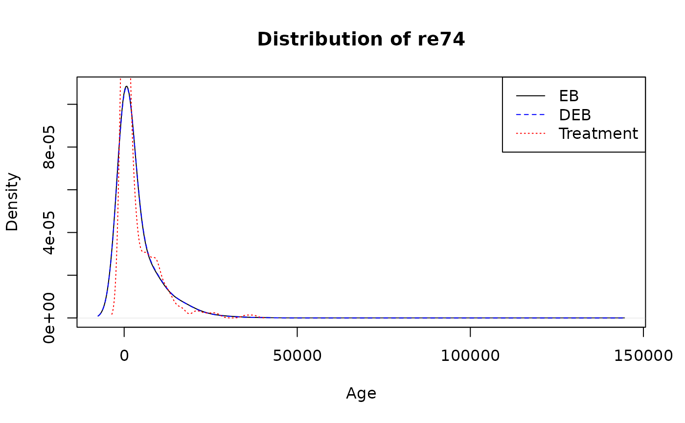

Compare balancing weights.

plot(x = bal_standard$w,
     y = bal_quant$g, 
     xlab = "EB", ylab = "DEB", main = "Comparison of EB and DEB weights",
     xlim = c(0, 1.2), ylim = c(0, 1.2))

Compare estimates of ATT using EB and DEB.

c(EB = with(LaLonde, mean(re78[treat == 1]) - weighted.mean(re78[treat == 0], bal_standard$w)),
  DEB = with(LaLonde, mean(re78[treat == 1]) - weighted.mean(re78[treat == 0], bal_quant$g)))
#>        EB       DEB 
#> -378.4217 -392.0171

Compare QTT(0.5) using EB and DEB.

c(EB = with(LaLonde, median(re78[treat == 1]) - weightedMedian(re78[treat == 0], bal_standard$w)),
  DEB = with(LaLonde, median(re78[treat == 1]) - weightedMedian(re78[treat == 0], bal_quant$g)))
#>       EB      DEB 
#> 72.39014 35.93408

Compare QTT(\(\alpha\)) where \(\alpha \in \{0.1, ..., 0.9\}\).

probs_qtt <- seq(0.1, 0.9, 0.1)
data.frame(
  EB = with(LaLonde, 
            quantile(re78[treat == 1], probs_qtt) - weightedQuantile(re78[treat == 0], bal_standard$w, probs_qtt)),
  DEB = with(LaLonde, 
            quantile(re78[treat == 1], probs_qtt) - weightedQuantile(re78[treat == 0], bal_quant$g, probs_qtt))
)
#>              EB         DEB
#> 10%     0.00000     0.00000
#> 20%     0.00000     0.00000
#> 30%   788.12509   784.81613
#> 40%   265.73521   261.63315
#> 50%    72.39014    35.93408
#> 60%   156.65605   -20.31025
#> 70%  -549.49531  -669.21504
#> 80%  -498.36777  -498.36777
#> 90% -2818.06621 -2818.06621

ATT with CBPS and DPS [work in progress]

m0 <- CBPS(formula = treat ~ age + educ + black + hisp + married + nodegr + re74,
           data = LaLonde)
#> [1] "Finding ATT with T=1 as the treatment.  Set ATT=2 to find ATT with T=0 as the treatment"

m1 <- joint_calib_cbps(formula_means = ~ age + educ + black + hisp + married + nodegr,
                       formula_quantiles = ~ re74, 
                       probs = 0.5,
                       treatment =  ~ treat,
                       data = LaLonde)

Maciej Beręsewicz

Theory

Distributional entropy balancing

Distributional propensity score method

Packages

ATT with entropy balancing and other methods

Single variable: age

More variables

More variables: all variables

ATT with CBPS and DPS [work in progress]

Single variable: `age`