Blocking records for deduplication
Maciej Beręsewicz
Source:vignettes/v1-deduplication.Rmd
v1-deduplication.RmdSetup
Read required packages
Read the RLdata500 data from the RecordLinkage
package from the dblink
Github repository.
df <- read.csv("https://raw.githubusercontent.com/cleanzr/dblink/dc3dd0daf55f8a303863423817a0f0042b3c275a/examples/RLdata500.csv")
setDT(df)
head(df)
#>    fname_c1 fname_c2 lname_c1 lname_c2    by    bm    bd rec_id ent_id
#>      <char>   <char>   <char>   <char> <int> <int> <int>  <int>  <int>
#> 1:  CARSTEN     <NA>    MEIER     <NA>  1949     7    22      1     34
#> 2:     GERD     <NA>    BAUER     <NA>  1968     7    27      2     51
#> 3:   ROBERT     <NA> HARTMANN     <NA>  1930     4    30      3    115
#> 4:   STEFAN     <NA>    WOLFF     <NA>  1957     9     2      4    189
#> 5:     RALF     <NA>  KRUEGER     <NA>  1966     1    13      5     72
#> 6:  JUERGEN     <NA>   FRANKE     <NA>  1929     7     4      6    142
This dataset contains 500 with 450 entities.
Blocking for deduplication
Now we create a new column that concatenates the information in each row.
df[, id_count :=.N, ent_id] ## how many times given unit occurs
df[is.na(fname_c2), fname_c2:=""]
df[is.na(lname_c2), lname_c2:=""]
df[, bm:=sprintf("%02d", bm)] ## add leading zeros to month
df[, bd:=sprintf("%02d", bd)] ## add leading zeros to month
df[, txt:=tolower(paste0(fname_c1,fname_c2,lname_c1,lname_c2,by,bm,bd))]
head(df)
#>    fname_c1 fname_c2 lname_c1 lname_c2    by     bm     bd rec_id ent_id
#>      <char>   <char>   <char>   <char> <int> <char> <char>  <int>  <int>
#> 1:  CARSTEN             MEIER           1949     07     22      1     34
#> 2:     GERD             BAUER           1968     07     27      2     51
#> 3:   ROBERT          HARTMANN           1930     04     30      3    115
#> 4:   STEFAN             WOLFF           1957     09     02      4    189
#> 5:     RALF           KRUEGER           1966     01     13      5     72
#> 6:  JUERGEN            FRANKE           1929     07     04      6    142
#>    id_count                    txt
#>       <int>                 <char>
#> 1:        1   carstenmeier19490722
#> 2:        2      gerdbauer19680727
#> 3:        1 roberthartmann19300430
#> 4:        1    stefanwolff19570902
#> 5:        1    ralfkrueger19660113
#> 6:        1  juergenfranke19290704
In the next step we use the newly created column in the
blocking function. If we specify verbose, we get
information about the progress.
set.seed(2024)
df_blocks <- blocking(x = df$txt, ann = "nnd", verbose = 1, graph = TRUE)
#> ===== creating tokens =====
#> ===== starting search (nnd, x, y: 500, 500, t: 429) =====
#> ===== creating graph =====
Results are as follows:
- based in
rnndescentwe have created 156 blocks, - it was based on 429 columns (2 character shingles),
- we have 93 blocks of 2 elements, 38 blocks of 3 elements, …, 3 block of 6 elements.
df_blocks
#> ========================================================
#> Blocking based on the nnd method.
#> Number of blocks: 156.
#> Number of columns used for blocking: 429.
#> Reduction ratio: 0.9952.
#> ========================================================
#> Distribution of the size of the blocks:
#>  2  3  4  5  6
#> 95 34 18  7  2
Structure of the object is as follows:
-
result- a data.table with identifiers and block IDs, -
method- the method used, -
deduplication– whether deduplication was applied, -
metrics- standard metrics and based on theigraph::comparemethods for comparing graphs (here NULL), -
colnames- column names used for the comparison, -
graph– anigraphobject mainly for visualisation.
str(df_blocks,1)
#> List of 7
#>  $ result       :Classes 'data.table' and 'data.frame':  255 obs. of  4 variables:
#>   ..- attr(*, ".internal.selfref")=<externalptr>
#>  $ method       : chr "nnd"
#>  $ deduplication: logi TRUE
#>  $ metrics      : NULL
#>  $ confusion    : NULL
#>  $ colnames     : chr [1:429] "86" "ap" "av" "bf" ...
#>  $ graph        :Class 'igraph'  hidden list of 10
#>  - attr(*, "class")= chr "blocking"
Plot connections
plot(df_blocks$graph, vertex.size=1, vertex.label = NA)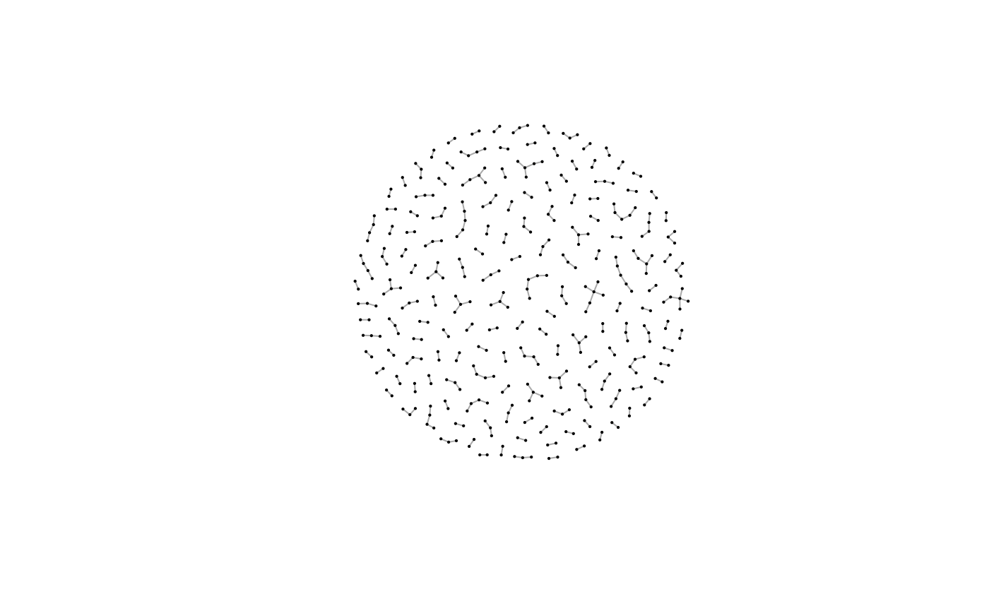
The resulting data.table has three columns:
-
x– reference dataset (i.e.df) – this may not contain all units ofdf, -
y- query (each row ofdf) – this may not contain all units ofdf, -
block– the block ID, -
dist– distance between objects.
head(df_blocks$result)
#>        x     y block       dist
#>    <int> <int> <num>      <num>
#> 1:     2    43     4 0.08074528
#> 2:     2   486     4 0.41023219
#> 3:     5   128    24 0.51333570
#> 4:     7    20     1 0.27246720
#> 5:     7    28     1 0.45405132
#> 6:     9   255    64 0.36754447
Create long data.table with information on blocks and
units from original dataset.
df_block_melted <- melt(df_blocks$result, id.vars = c("block", "dist"))
df_block_melted_rec_block <- unique(df_block_melted[, .(rec_id=value, block)])
head(df_block_melted_rec_block)
#>    rec_id block
#>     <int> <num>
#> 1:      2     4
#> 2:      5    24
#> 3:      7     1
#> 4:      9    64
#> 5:     10    49
#> 6:     11   107
We add block information to the final dataset.
df[df_block_melted_rec_block, on = "rec_id", block_id := i.block]
head(df)
#>    fname_c1 fname_c2 lname_c1 lname_c2    by     bm     bd rec_id ent_id
#>      <char>   <char>   <char>   <char> <int> <char> <char>  <int>  <int>
#> 1:  CARSTEN             MEIER           1949     07     22      1     34
#> 2:     GERD             BAUER           1968     07     27      2     51
#> 3:   ROBERT          HARTMANN           1930     04     30      3    115
#> 4:   STEFAN             WOLFF           1957     09     02      4    189
#> 5:     RALF           KRUEGER           1966     01     13      5     72
#> 6:  JUERGEN            FRANKE           1929     07     04      6    142
#>    id_count                    txt block_id
#>       <int>                 <char>    <num>
#> 1:        1   carstenmeier19490722       NA
#> 2:        2      gerdbauer19680727        4
#> 3:        1 roberthartmann19300430       NA
#> 4:        1    stefanwolff19570902       NA
#> 5:        1    ralfkrueger19660113       24
#> 6:        1  juergenfranke19290704       NA
We can check in how many blocks the same entities
(ent_id) are observed. In our example, all the same
entities are in the same blocks.
df[, .(uniq_blocks = uniqueN(block_id)), .(ent_id)][, .N, uniq_blocks]
#>    uniq_blocks     N
#>          <int> <int>
#> 1:           1   450
We can visualise the distances between units stored in the
df_blocks$result data set. Clearly we a mixture of two
groups: matches (close to 0) and non-matches (close to 1).
hist(df_blocks$result$dist, xlab = "Distances", ylab = "Frequency", breaks = "fd",
     main = "Distances calculated between units")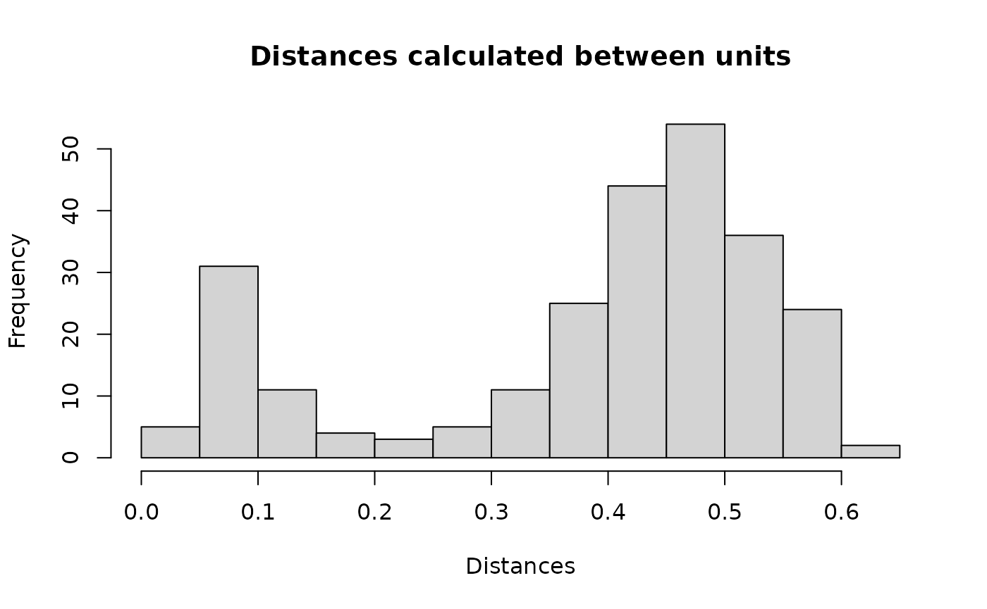
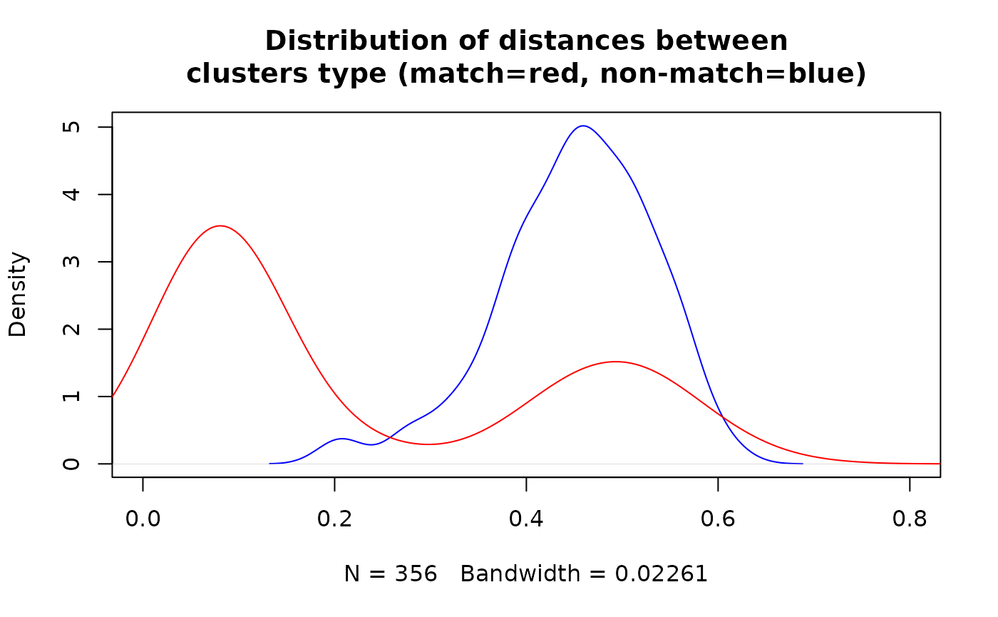
Finally, we can visualise the result based on the information whether block contains matches or not.
df_for_density <- copy(df_block_melted[block %in% df$block_id])
df_for_density[, match:= block %in% df[id_count == 2]$block_id]

plot(density(df_for_density[match==FALSE]$dist), col = "blue", xlim = c(0, 0.8),
     main = "Distribution of distances between\nclusters type (match=red, non-match=blue)")
lines(density(df_for_density[match==TRUE]$dist), col = "red", xlim = c(0, 0.8))