Blocking records for record linkage

Setup

Read required packages

library(blocking)
library(reclin2)
#> Loading required package: data.table
library(data.table)
library(rnndescent)

Data

Read the example data from the tutorial on the reclin package on the URos 2021 Conference. The data sets are from ESSnet on Data Integration as stated in the repository:

These totally fictional data sets are supposed to have captured details of
persons up to the date 31 December 2011.  Any years of birth captured as 2012
are therefore in error.  Note that in the fictional Census data set, dates of
birth between 27 March 2011 and 31 December 2011 are not necessarily in error.

Census: A fictional data set to represent some observations from a
        decennial Census
CIS: Fictional observations from Customer Information System, which is
        combined administrative data from the tax and benefit systems

In the dataset census all records contain a person_id. For some of the records
in cis the person_id is also available. This information can be used to
evaluate the linkage (assuming these records from the cis are representable 
all records in the cis).

census <- fread("https://raw.githubusercontent.com/djvanderlaan/tutorial-reclin-uros2021/main/data/census.csv")
cis <- fread("https://raw.githubusercontent.com/djvanderlaan/tutorial-reclin-uros2021/main/data/cis.csv")

census object has 25343 rows and 9,
cis object has 25343 rows and 9.

Census data

head(census)
#>       person_id pername1 pername2    sex dob_day dob_mon dob_year
#>          <char>   <char>   <char> <char>   <int>   <int>    <int>
#> 1: DE03US001001    COUIE    PRICE      M       1       6     1960
#> 2: DE03US001002    ABBIE    PVICE      F       9      11     1961
#> 3: DE03US001003    LACEY    PRICE      F       7       2     1999
#> 4: DE03US001004   SAMUEL    PRICE      M      13       4     1990
#> 5: DE03US001005   JOSEPH    PRICE      M      20       4     1986
#> 6: DE03US001006     JOSH    PRICE      M      14       2     1996
#>           enumcap enumpc
#>            <char> <char>
#> 1: 1 WINDSOR ROAD DE03US
#> 2: 1 WINDSOR ROAD DE03US
#> 3: 1 WINDSOR ROAD DE03US
#> 4: 1 WINDSOR ROAD DE03US
#> 5: 1 WINDSOR ROAD DE03US
#> 6: 1 WINDSOR ROAD DE03US

CIS data

head(cis)
#>    person_id pername1 pername2    sex dob_day dob_mon dob_year
#>       <char>   <char>   <char> <char>   <int>   <int>    <int>
#> 1:      <NA>   HAYDEN     HALL      M      NA       1       NA
#> 2:      <NA>    SEREN ANDERSON      F       1       1       NA
#> 3:      <NA>    LEWIS    LEWIS      M       1       1       NA
#> 4:      <NA> HARRISON   POSTER      M       5       1       NA
#> 5:      <NA> MUHAMMED   WATSUN      M       7       1       NA
#> 6:      <NA>     RHYS THOMPSON      M       7       1       NA
#>               enumcap  enumpc
#>                <char>  <char>
#> 1:   91 CLARENCE ROAD PO827ER
#> 2:     24 CHURCH LANE LS992DB
#> 3:     53 CHURCH ROAD  M432ZZ
#> 4:  19 HIGHFIELD ROAD  SW75TG
#> 5: 17 VICTORIA STREET        
#> 6: 1 SPRINGFIELD ROAD SW540RB

We need to create new columns that concatanates variables from pername1 to enumpc. In the first step we replace NAs with ''.

census[, ":="(dob_day=as.character(dob_day), dob_mon=as.character(dob_mon), dob_year=as.character(dob_year))]
cis[, ":="(dob_day=as.character(dob_day), dob_mon=as.character(dob_mon),dob_year=as.character(dob_year))]

census[is.na(dob_day), dob_day := ""]
census[is.na(dob_mon), dob_mon := ""]
census[is.na(dob_year), dob_year := ""]
cis[is.na(dob_day), dob_day := ""]
cis[is.na(dob_mon), dob_mon := ""]
cis[is.na(dob_year), dob_year := ""]

census[, txt:=paste0(pername1, pername2, sex, dob_day, dob_mon, dob_year, enumcap, enumpc)]
cis[, txt:=paste0(pername1, pername2, sex, dob_day, dob_mon, dob_year, enumcap, enumpc)]

Linking datasets

Using basic functionalities of `blocking` package

The goal of this exercise is to link units from the CIS dataset to the CENSUS dataset.

set.seed(2024)
result1 <- blocking(x = census$txt, y = cis$txt, verbose = 1, n_threads = 8)
#> ===== creating tokens =====
#> ===== starting search (nnd, x, y: 25343, 24613, t: 1072) =====
#> ===== creating graph =====

Distribution of distances for each pair.

hist(result1$result$dist, main = "Distribution of distances between pairs", xlab = "Distances")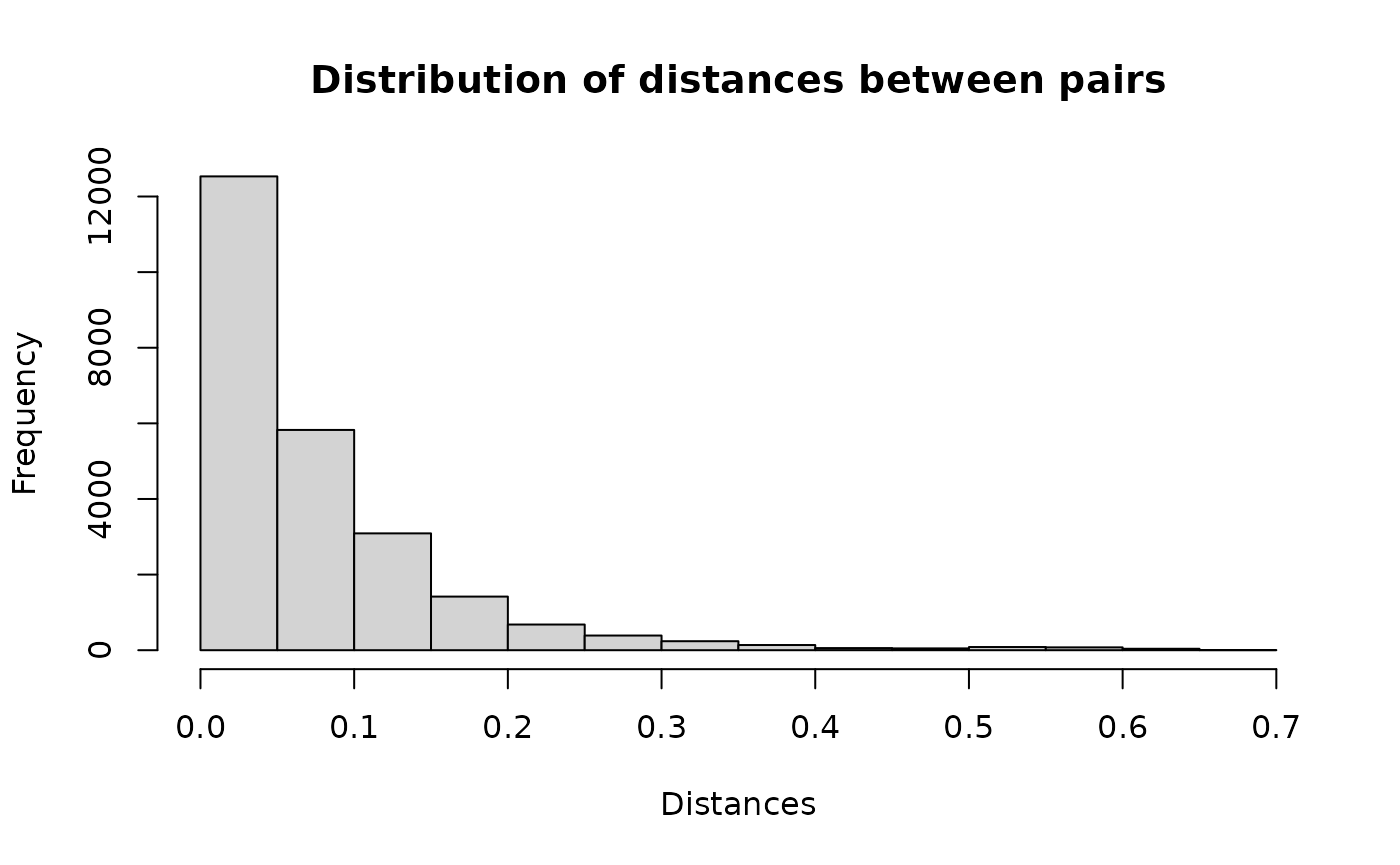

Example pairs.

head(result1$result, n= 10)
#>         x     y block          dist
#>     <int> <int> <num>         <num>
#>  1:     1  8152  8023  2.941167e-02
#>  2:     2  8584  8447  4.878050e-02
#>  3:     3 20590 19948  1.290381e-02
#>  4:     4 18456 17945  7.158583e-02
#>  5:     5 17257 16810  5.370837e-02
#>  6:     6 19868 19273  5.675775e-02
#>  7:     7 11183 10963 -1.192093e-07
#>  8:    10  9370  9212  8.233702e-02
#>  9:    11  7247  7143  4.881024e-02
#> 10:    12 10622 10424  2.777779e-02

Let’s take a look at the first pair. Obviously there is a typo in the pername1, but all the other variables are the same, so it appears to be a match.

cbind(t(census[1, 1:9]), t(cis[8152, 1:9]))
#>           [,1]             [,2]            
#> person_id "DE03US001001"   NA              
#> pername1  "COUIE"          "LOUIE"         
#> pername2  "PRICE"          "PRICE"         
#> sex       "M"              "M"             
#> dob_day   "1"              "1"             
#> dob_mon   "6"              "6"             
#> dob_year  "1960"           "1960"          
#> enumcap   "1 WINDSOR ROAD" "1 WINDSOR ROAD"
#> enumpc    "DE03US"         "DE03US"

Assessing the quality

For some records, we have information about the correct linkage. We can use this information to evaluate our approach, but note that the information for evaluating quality is described in detail in the other vignette.

matches <- merge(x = census[, .(x=1:.N, person_id)],
                 y = cis[, .(y = 1:.N, person_id)],
                 by = "person_id")
matches[, block:=1:.N]
head(matches)
#> Key: <person_id>
#>        person_id     x     y block
#>           <char> <int> <int> <int>
#> 1:  DE03US012003    20 21256     1
#> 2:  DE03US015002    35  9524     2
#> 3:  DE03US019002    44  6754     3
#> 4:  DE03UT043001    81 17312     4
#> 5: DE125LU002001    98 12386     5
#> 6: DE125LU016001   126 11309     6

So in our example we have 971 pairs.

set.seed(2024)
result2 <- blocking(x = census$txt, y = cis$txt, verbose = 1,
                    true_blocks = matches[, .(x, y, block)], n_threads = 8)
#> ===== creating tokens =====
#> ===== starting search (nnd, x, y: 25343, 24613, t: 1072) =====
#> ===== creating graph =====

Let’s see how our approach handled this problem.

result2
#> ========================================================
#> Blocking based on the nnd method.
#> Number of blocks: 23795.
#> Number of columns used for blocking: 1072.
#> Reduction ratio: 1.0000.
#> ========================================================
#> Distribution of the size of the blocks:
#>     2     3     4     5 
#> 23002   769    23     1 
#> ========================================================
#> Evaluation metrics (standard):
#>      recall   precision         fpr         fnr    accuracy specificity 
#>     98.6612     98.6612      0.0007      1.3388     99.9987     99.9993

It seems that the default parameters of the NND method result in an FNR of 1.34%. We can see if increasing the number of k (and thus max_candidates) as suggested in the Nearest Neighbor Descent vignette will help.

set.seed(2024)
ann_control_pars <- controls_ann()
ann_control_pars$nnd$epsilon <- 0.2


result3 <- blocking(x = census$txt, y = cis$txt, verbose = 1, 
                    true_blocks = matches[, .(x, y, block)], n_threads = 8, 
                    control_ann = ann_control_pars)
#> ===== creating tokens =====
#> ===== starting search (nnd, x, y: 25343, 24613, t: 1072) =====
#> ===== creating graph =====

Changing the epsilon search parameter from 0.1 to 0.2 decreased the FDR to 0.5%.

result3
#> ========================================================
#> Blocking based on the nnd method.
#> Number of blocks: 23950.
#> Number of columns used for blocking: 1072.
#> Reduction ratio: 1.0000.
#> ========================================================
#> Distribution of the size of the blocks:
#>     2     3     4     5 
#> 23303   632    14     1 
#> ========================================================
#> Evaluation metrics (standard):
#>      recall   precision         fpr         fnr    accuracy specificity 
#>     99.4851     99.4851      0.0003      0.5149     99.9995     99.9997

Finally, compare the NND and HNSW algorithm for this example.

result4 <- blocking(x = census$txt, y = cis$txt, verbose = 1, 
                    true_blocks = matches[, .(x, y, block)], n_threads = 8, 
                    ann = "hnsw", seed = 2024)
#> ===== creating tokens =====
#> ===== starting search (hnsw, x, y: 25343, 24613, t: 1072) =====
#> ===== creating graph =====

It seems that the HNSW algorithm performed better with 0.51% FNR.

result4
#> ========================================================
#> Blocking based on the hnsw method.
#> Number of blocks: 23994.
#> Number of columns used for blocking: 1072.
#> Reduction ratio: 1.0000.
#> ========================================================
#> Distribution of the size of the blocks:
#>     2     3     4     5 
#> 23390   590    13     1 
#> ========================================================
#> Evaluation metrics (standard):
#>      recall   precision         fpr         fnr    accuracy specificity 
#>     99.4851     99.4851      0.0003      0.5149     99.9995     99.9997

Compare results

Finally, we can compare the results of two ANN algorithms. The overlap between neighbours is given by

c("no tuning" = mean(result2$result[order(y)]$x == result4$result[order(y)]$x)*100,
  "with tuning" = mean(result3$result[order(y)]$x == result4$result[order(y)]$x)*100)
#>   no tuning with tuning 
#>    99.03303    99.76435